Quickstart#
import pytometry as pm
import readfcs
import anndata
Read fcs file example from the readfcs package. The fcs file was part of the following reference and originally deposited on the FlowRepository.
path_data = readfcs.datasets.Oetjen18_t1()
adata = pm.io.read_fcs(path_data)
assert isinstance(adata, anndata._core.anndata.AnnData)
Next, we split the data matrix into the marker intensity part and the FSC/SSC part. Moreover, we move all height related features to the .obs part of the anndata file. Notably. the function split_signal checks if a feature name is either FSC/SSC or whether a name endswith -A for area related features and -H for height related features.
pm.pp.split_signal(adata, var_key="channel")
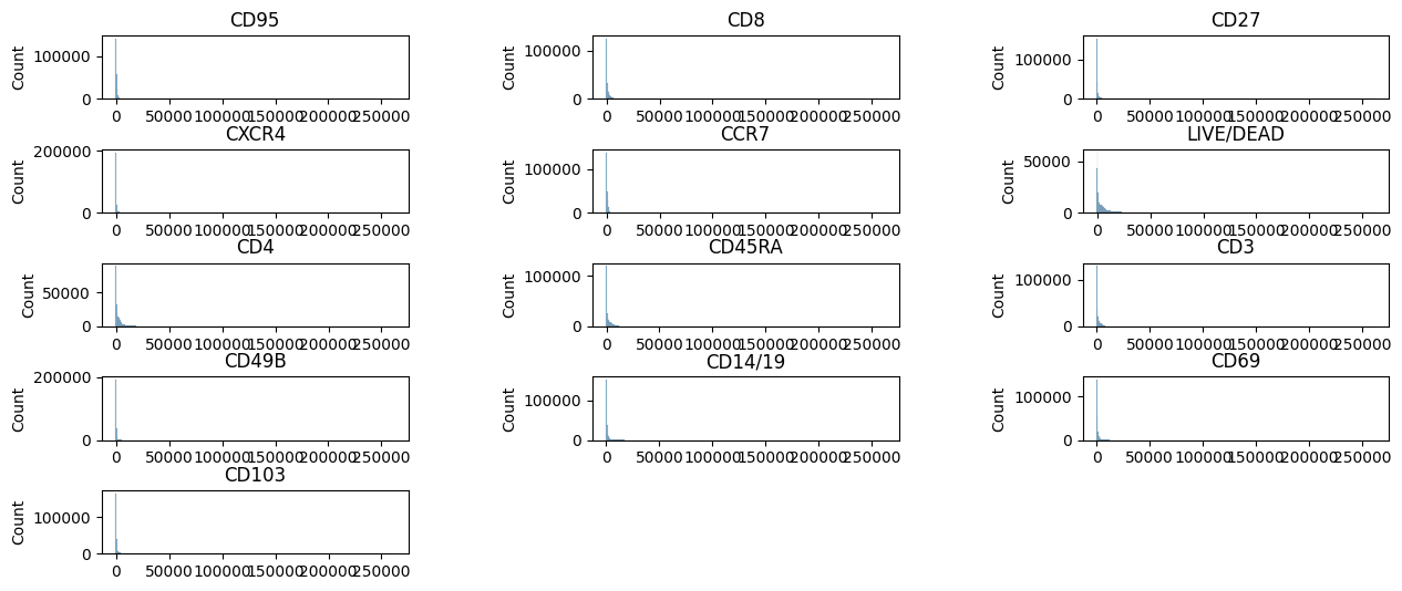
We can plot the fluorescent marker intensity distribution with the plotdata function.
pm.pl.plotdata(adata)

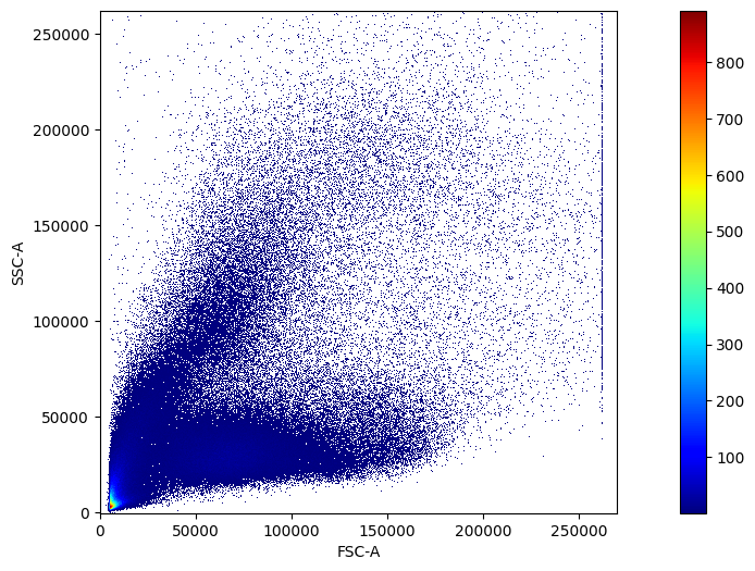
For 2D distribution plots, we use the scatter_density function.
pm.pl.scatter_density(adata, x_lim=[-1, 2.7e5])

pm.pp.compensate(adata)
adata_arcsinh = pm.tl.normalize_arcsinh(adata, cofactor=150, inplace=False)
adata_biexp = pm.tl.normalize_biExp(adata, inplace=False)
adata_logicle = pm.tl.normalize_logicle(adata, inplace=False)
Save data to HDF5 file format.
adata.write("example.h5ad")